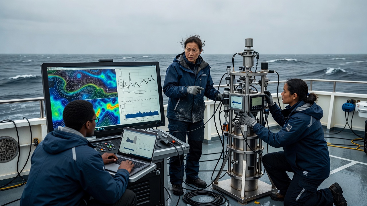
Start with a changing physical system
An ocean model represents relationships among velocity, pressure, temperature, salinity and other quantities. Its equations describe how momentum, mass, heat and salt evolve under specified assumptions. Earth’s rotation, gravity, winds and exchanges at the surface shape the result. The seafloor and coastline constrain where water can move. A model is therefore more than a statistical fill between dots, although statistical methods often help connect its state with observations.
The ocean contains motions far smaller than a practical global grid. Their collective effects must often be parameterised rather than explicitly resolved. Vertical mixing is one important example. Different parameterisations can produce different water-column structures and circulation patterns even when the models use similar observations. Knowing the model configuration helps explain those differences before deciding which map looks more convincing.
A grid is a choice, not a guarantee
The horizontal grid divides the domain into computational cells, while vertical coordinates represent depth using layers or other arrangements. Finer spacing can allow smaller features to emerge, but it increases computational demands and does not remove errors in forcing, bathymetry or boundary conditions. Effective resolution is coarser than one grid cell, because a feature generally needs several cells to be represented meaningfully.
A coastal model of the Bay of Biscay may focus on shelf processes that a global model handles only broadly. A regional model also needs information at its open boundaries. Those boundary fields may come from a larger model, carrying both useful structure and inherited errors. Features in the Mediterranean Sea require attention to narrow passages and exchanges, which illustrates why configuration matters as much as an attractive nominal resolution.
Forcing sets the ocean in motion
Models use atmospheric information such as wind stress, heat exchange and freshwater fluxes. Rivers, sea ice and tides may also be included, depending on the system and purpose. Atmospheric products from organisations such as ECMWF provide important inputs, but uncertainty in a wind event can propagate into the estimated current. Incorrect freshwater input can alter density structure and mixing near a coast.
Initial conditions also matter. A forecast begins from an estimate of the present ocean, not a perfectly known state. Some errors grow rapidly, while larger-scale patterns may remain predictable for longer. Forecast usefulness therefore depends on the variable, region, season and lead time. There is no single universal horizon beyond which every ocean prediction suddenly becomes invalid.
Assimilation brings observations into the estimate
Data assimilation combines a model-based prior estimate with observations, taking account of their uncertainties and relationships. Altimetry can constrain sea-surface height; Argo profiles can constrain temperature and salinity below the surface. Other observations may enter according to the system’s design. The adjustment can influence nearby variables and locations through the assumed error structure and the model dynamics.
Assimilation is not a rule that every measurement must be matched exactly. A suspect observation may be rejected, and a valid observation still has uncertainty and representativeness limits. A thermometer samples a particular place and time; a model cell represents a volume and a discretised state. Comparing the two responsibly requires attention to that mismatch, not merely subtracting one displayed number from another.
Analysis, forecast and reanalysis differ
An analysis estimates the ocean state using observations available to a particular production system. A forecast then evolves an initial estimate forward. A reanalysis revisits an extended historical period using a relatively consistent modelling and assimilation framework, often benefiting from later data processing. These labels describe workflows, not an automatic ranking of truth. Product documentation explains which observations were available and which assumptions changed.
Copernicus Marine provides access to different ocean products, while systems associated with Mercator Ocean International, HYCOM and ECCO illustrate distinct modelling and estimation approaches. They should not be treated as interchangeable datasets. Check whether a product includes tides, how it defines surface velocity, how frequently it is updated and whether the displayed field is an instantaneous state or a time average.
Validation must leave room for disagreement
Independent observations are especially valuable for evaluation. If a satellite record was assimilated, agreement with that same record is not a fully independent test. Withheld drifters, moorings or profiles may reveal regional and seasonal weaknesses. Bias, root-mean-square error and ensemble spread answer different questions; no single statistic summarises every useful aspect of model skill.
For readers, the practical conclusion is simple. A complete grid offers coherence, not omniscience. Look for validation reports, examine the relevant region and depth, and ask whether the product was designed for your question. A basin-scale circulation estimate can be scientifically useful while remaining unsuitable for a harbour manoeuvre or a person’s safety decision at a beach.